Guest Essay
Time to engage in measurement uncertainty
In the ongoing "War of Words" in the Lab, it's time to hear another voice. Dr. Dietmar Stockl, an expert from across the Atlantic, provides us with a detailed essay explaining how measurement uncertainty can be useful to the laboratory - and even co-exist with Total Error.
- Introduction
- Calculation of measurement uncertainty (adapted from the NIST website)
- GUM calculations “lightweight”
- Applications
- So why the fuss about GUM, there’s nothing new?
- Laboratory Approach using available data
- Limitations of GUM
- A note on Quality Control
- References
- Internet Resources
September 2008
Dietmar Stöckl
STT Consulting
Abraham Hansstraat 11
B-9667 Horebeke, Belgium
e-mail: This email address is being protected from spambots. You need JavaScript enabled to view it.
Introduction
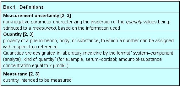
Measurement results are inherently variable due to the influences of random and systematic effects. This variability must be quantified so that the user of the results has knowledge of their reliability. The Guide to the Expression of Uncertainty in Measurement (GUM) [1] provides general rules for quantifying measurement variability. Measurement variability quantified by the rules of GUM is called measurement uncertainty (see also Box 1 for definitions [2, 3]). Because of confusion what GUM is really about and the many personal interpretations of GUM, the concept is introduced by use of original GUM citations (indicated by “quotation marks” and paragraph number).
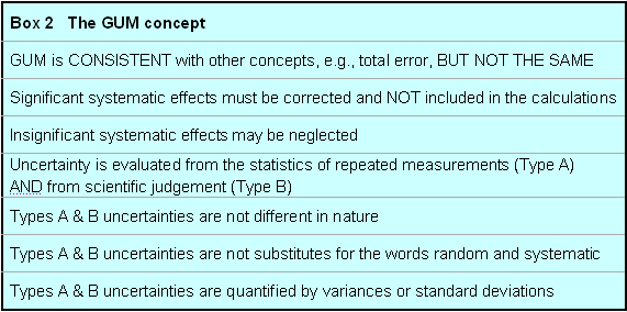
One of the most important aspects of the GUM concept is that “it is assumed that the result of a measurement has been corrected for all recognized significant systematic effects and that every effort has been made to identify such effects” (3.2.4). However, “the result of a measurement after correction for recognized systematic effects is still only an estimate of the value of a measurand because of the uncertainty arising from random effects and from imperfect correction of the result for systematic effects” (3.3.1). Thus, “in general, the result of a measurement is only an approximation or estimate of the value of the measurand and thus is complete only when accompanied by a statement of the uncertainty of that estimate” (3.1.2). Measurement uncertainty is evaluated by two different methods; “Type A: method of evaluation of uncertainty by the statistical analysis of series of observations” (2.3.2); “Type B: method of evaluation of uncertainty by means other than the statistical analysis of series of observations” (2.3.3). “Type B is evaluated by scientific judgement based on all the available information on the possible variation of the measurand. The pool of information may include i) previous measurement data; ii) experience with or general knowledge of the behaviour and properties of relevant materials and instruments; iii) manufacturer’s specifications; iv) data provided in calibration and other certificates; v) uncertainties assigned to reference data taken from handbooks” (4.3). “The purpose of the Type A and Type B classification is to indicate the two different ways of evaluating uncertainty components and is for convenience of discussion only; the classification is not meant to indicate that there is any difference in the nature of the components resulting from the two types of evaluation. Both types of evaluation are based on probability distributions, and the uncertainty components resulting from either type are quantified by means of variances or standard deviations” (3.3.4). Note, “these categories are not substitutes for the words random and systematic” (3.3.3). “Type A uncertainty is obtained from a probability density function derived from an observed frequency distribution, while Type B uncertainty is obtained from an assumed probability density function based on the degree of belief that an event will occur” (3.3.5). It should be stressed that “the definition of uncertainty of measurement is not inconsistent with other concepts of uncertainty of measurement, such as a measure of the possible error in the estimated value of the measurand as provided by the result of a measurement. Nevertheless, “whichever concept of uncertainty is adopted, an uncertainty component is always evaluated using the same data and related information” (2.2.4). See Box 2 for a summary of the GUM concept.
Calculation of measurement uncertainty (adapted from the NIST website)
CAUTION: Some heavy stuff ahead. If you wish, continue below.
Before starting an uncertainty calculation, one has to define the measurement equation. Usually, the quantity Y (called the measurand), is not measured directly, but is determined from N other quantities X1, X2, . . . , XN through a functional relation f, often called the measurement equation: Y= f(X1, X2, . . . , XN). Included among the quantities Xi are corrections (or correction factors), as well as other sources of variability, such as different observers, instruments, samples and sampling, laboratories, and times at which observations are made. Thus, the function f of the above equation should express not simply a physical law but a measurement process, and in particular, it should contain all quantities that can contribute a significant uncertainty to the measurement result. An estimate of the measurand or output quantity Y, denoted by y, is obtained from the above equation using input estimates x1, x2, . . . , xN for the values of the N input quantities X1, X2, . . . , XN. Thus, the output estimate y (= result), is given by y= f(x1, x2, . . . , xN). The uncertainty of the measurement result y arises from the uncertainties u(xi) (or ui) of the input estimates xi that enter the equation. The combined standard uncertainty of the measurement result y, designated by uc(y) is the positive square root of the estimated variance uc2(y) obtained from

This equation is based on a first-order Taylor series approximation of the measurement equation and is referred to as the law of propagation of uncertainty. The partial derivatives of f are often referred to as sensitivity coefficients and u(xi, xj) is the covariance associated with xi and xj. The partial derivatives of f with respect to the Xi are equal to the partial derivatives of f with respect to the Xi evaluated at Xi = xi; u(xi) is the standard uncertainty associated with the input estimate xi. Note, standard uncertainties of Type A equal standard deviations typically estimated in the laboratory (u(xi) = SD(xi)). If the probability distribution of y and its combined standard uncertainty uc(y) is approximately normal (Gaussian) then the interval y ± uc(y) should encompass ~68% of the values that could reasonably be attributed to Y (Y= y ± uc(y)). If other confidence levels are desired, the standard uncertainty may be expanded (expanded uncertainty: U = k uc) by use of a coverage factor, k (e.g., 2 or 3: approximate confidence of 95 or >99%).
GUM uncertainty calculations can be made as sophisticated as desired. I will present here only the “lightweight” version. At the end, a laboratory approach is given for estimating measurement uncertainty using available data.
However, if you are required to do in-depth GUM calculations (manufacturer; in-house method developer), it is recommended to consult the internet resources given below and to purchase the GUM.
GUM calculations “lightweight”
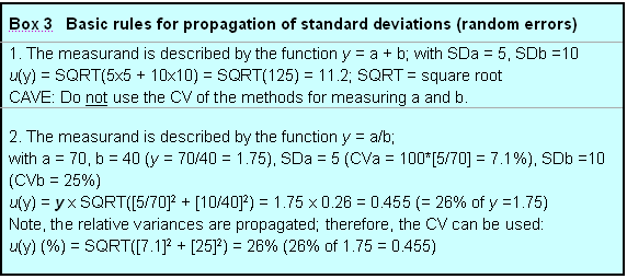
Boiled down, GUM is about propagation of standard deviations/variances. This is also part of standard clinical chemistry textbooks [4]. The 2 simpliest cases of error propagation will be addressed, namely, sums and multiplications/divisions (both follow the same rule).
1. The measurand is described by the function y = a + b; with SDa = 5, SDb =10
u(y) = SQRT(5x5 + 10x10) = SQRT(125) = 11.2; SQRT = square root
CAVE: Do not use the CV of the methods for measuring a and b.
2. The measurand is described by the function y = a/b;
with a = 70, b = 40 (y = 70/40 = 1.75), SDa = 5 (CVa = 100*[5/70] = 7.1%), SDb =10 (CVb = 25%)
u(y) = y x SQRT([5/70]2 + [10/40]2) = 1.75 x 0.26 = 0.455 (= 26% of y =1.75)
Note, the relative variances are propagated; therefore, the CV can be used:
u(y) (%) = SQRT([7.1]2 + [25]2) = 26% (26% of 1.75 = 0.455)
These equations shall be applied to the calculation of the uncertainty of the anion gap and the creatinine clearance.
Applications [see also 4]
Anion gap (AG)
AG = ([Na+]+[K+]) - ([Cl-]+[HCO3-])
For daily practice, potassium is frequently ignored, leaving the equation:
AG = ([Na+]) - ([Cl-]+[HCO3-]) mmol/L
For example: AG = 140 – (106 + 22) = 12 mmol/L
SD[Na+] = 1.3 mmol/L; SD[Cl-] = 1.2 mmol/L; SD[HCO3-] = 0.7 mmol/L
SD[AG] = SQRT(1.32 + 1.22 + 0.72) = 1.9 mmol/L
This value equals the standard uncertainty for the anion gap:
u(AG) = 1.9 mmol/L; using a coverage factor of 2 (approximately 95% probability), the expanded uncertainty is U = 3.8 mmol/L. This is equivalent to a total error (TE), in the absence of a systematic error (SE), calculated as 2 times the random error (RE): TE = 2 x RE.
Creatinine clearance
Ccr = (U x V)/S mL/min
Creatinine clearance (Ccr; mL/min); urine creatinine (U; µmol/L); volume urine/minute (V; mL/min); serum creatinine (S; µmol/L)
With CV(U) = 3%; CV(V) = 10%; CV(S) = 3%
CV(Ccr) = SQRT(32 + 102 + 32) = 11%
At a Ccr of 80 mL/min, u(Ccr) = 8.8 mL/min (= 11% of 80 mL/min)
So why the fuss about GUM, there’s nothing new?
While GUM computations may be simple, the GUM philosophy encourages the analyst to look “what is behind the input data”, in particular, to address the Type B uncertainty. The problem with the anion gap, for example, is that it may widely vary with insstruments. Therefore, care should be taken that the involved measurement procedures are correctly standardized and the correct reference interval is used for its interpretation (5, 6). This line of thought is continued in the example below.
Laboratory approach using available data
|
| Analytical specificity | Cross reactivity data, but no indication of their relevance for patients’ specimens. |
| Interference | Interference limit 10% (concentrations given for lipids, etc). No interference with common drugs. |
| Linearity | Limit 10% |
| Recovery | Limit 10% |
| Method comparison | Acceptable slope: 0.9 - 1.1 |
| Limit of detection (LoD) | 0.1 nmol/L |
| Quantitation limit (CV = 20%) | 0.4 nmol/L |
| Reportable range range (from LoD to calibration maximum) | 0.1 - 60 nmol/L |
| Expected values |
Male: 10 - 28 nmol/L |
| Stability data calibrator and reagent lots | Some decline during maximum recommended time (no limits given). |
| Lot-to-lot criteria calibrators and reagents | No information available. |

Scientific information
Consultation of the scientific literature revealed the risk of considerable sample related effects, in particular, for females (7). The incidence of antibody interference seems to be low (8, 9), while interferences due to cross-reactivity seem to be more common (10 - 12). Interferences to consider are dehydroepiandrostenedione sulphate and testosterone conjugates.
Laboratory approach for estimating measurement uncertainty using all above information
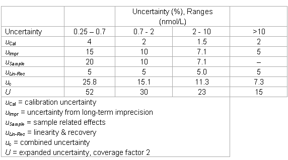
The laboratory could verify the imprecision data, but decided to modify the uncertainty estimates of the manufacturer in the following way:
- the uncertainty “point” estimates were converted into intervals and one range was added;
- the estimate in the low range was expanded for sample related effects and considering the quantitation limit of the assay (total effect: factor of 2);
- the estimate in the low-medium range was expanded by sample-related effects (in the order of the total imprecision) and the imprecision was interpolated;
- an uncertainty of 5% was added in all ranges to account for recovery and linearity;
- the lower end of the working range was increased to 0.25 nmol/L (relative big difference between the LoD and the quantitation limit).
- A risk analysis was done for interferences and a policy was written.
- The trueness problem was discussed with the manufacturer and their rationale was accepted.
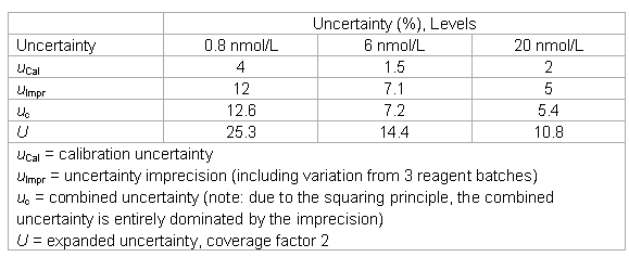
- The laboratory keeps the following uncertainty estimates in its files.
Beyond GUM
The long-term internal quality control data indicated a somewhat high lot-to-lot variation (u = 10%). The laboratory made total error calculations and simulations by introduction of biases. It found that biases of 10% changed the results “to be acted upon” by 50%. While this was deemed too high, no solution could be found. The laboratory increased its quality assurance efforts and introduced a quality control rule with an increased power.

Limitations of GUM
As outlined above, bias is not covered by the GUM calculations but needs to be corrected. However, the treatment of bias (existing or input in total error models) is vital to the laboratory. For example, to investigate the effect of reagent batch-to-batch variations on patient data. Figure 1 below shows a test with a batch-to-batch CVbb of 10% (= 10 at a value of 100) and a within-batch CVwb of 5%. It was created by simulating 20 random numbers with a SD of 10 and a mean of 100. Then, for each of the 20 values (batch means are indicated by bars), 20 random numbers were simulated with a SD of 5. The figure would represent quality control data obtained with a batch lasting 20 days and doing 1 QC sample a day. Further, it is assumed that the mean of the stable process is known to be 100.
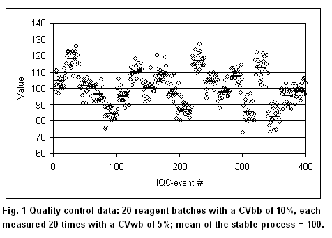
According to GUM, 2 possibilities exist. If the observation time is extended over all 20 batches, the biases of the individual batches become random and the total CVtot becomes 11.2%. The laboratory may decide to keep in its files that the process has an uncertainty of 11.2%, without considering the bias introduced when changing reagent batches. This, however, would give a false impression about the test performance, because the bias in each reagent batch may have a profound influence on diagnostic decisions (13). If the observation time is 2 batches, considerable systematic effects would be seen from time to time (batch 2, for example). This is the reasoning why GUM deprecates the distinction between “random” and “systematic”: it may depend on the observation time. According to GUM, one would correct the second batch giving a mean of 120 (bias = 20%). The laboratory, however, is usually unable to correct for batch-to-batch variations. Nevertheless, it needs to know the effect of a 20% bias on the patient results. If such a bias would increase the false positives by 50%, for example, it may require the manufacturer to tighten his batch-to-batch variations. Also, the laboratory needs a model that accounts for bias in order to select the appropriate quality control rules. Such a model, for example, is the total error approach used in the Westgard software products.
Contrary to the GUM philosophy, it is vital for the laboratory to distinguish between random and systematic effects. When systematic effects have to be taken into account, other concepts must be used for describing measurement variability, such as the total error concept. Thus, in my opinion, the different concepts are complementary and not contradictory. GUM alone, however, is unsufficient for managing real-world situations in the clinical laboratory.

A note on Quality control
The above example shows a dilemma of quality control: shall the laboratory use a CV of 11.2% or a CV of 5% as input value for the QC process? If a CV of 11.2% is chosen, typical QC rules seldom will give alarms. If a CV of 5% is chosen, typical QC rules will indicate problems regularly. But then, what to do? Currently, there is no easy answer to the problem. Obviously, for QC purposes, one could change the target value of the quality control sample, however, this changes nothing for the bias of the patient samples.
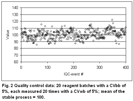
In the future, it would be desirable that manufacturers keep the between-batch variation in the same order as the within-batch variation. For comparison, Figure 2 shows a QC chart with CVbb = CVwb = 5%. The total CVtot is 7.1%.
References
- ISO/IEC Guide 98:1995. Guide to the expression of uncertainty in measurement (GUM). International Organization for Standardization: Geneva, 1995.
- ISO/IEC Guide 99:2007. International vocabulary of metrology – Basic and general concepts and associated terms (VIM). International Organization for Standardization: Geneva, 2007.
- JCGM 200:2008. International vocabulary of metrology – Basic and general concepts and associated terms (VIM). International Bureau of Weights and Measures (BIPM); Joint Committee for Guides in Metrology (JCGM): Paris, 2008 (electronic document freely available at: http://www.bipm.org/en/publications/guides/vim.html).
- Kringle RO. Statistical Procedures. In Burtis CA, Ashwood ER [eds]. Tietz Textbook of Clinical Chemistry, 2nd edition, Chapter 12, pages 419-422. Philadelphia: Saunders, 1994.
- Kraut JA, Madias NE. Serum anion gap: its uses and limitations in clinical medicine. Clin J Am Soc Nephrol 2007;2:162-74.
- Paulson WD, Roberts WL, Lurie AA, Koch DD, Butch AW, Aguanno JJ. Wide variation in serum anion gap measurements by chemistry analyzers. Am J Clin Pathol 1998;110:735-42.
- Taieb J, Mathian B, Millot F, Patricot MC, Mathieu E, Queyrel N, Lacroix I, Somma-Delpero C, Boudou P. Testosterone measured by 10 immunoassays and by isotope-dilution gas chromatography-mass spectrometry in sera from 116 men, women, and children. Clin Chem 2003;49:1381-95.
- Kuwahara A, Kamada M, Irahara M, Naka O, Yamashita T, Aono T. Autoantibody against testosterone in a woman with hypergonadotropic hypogonadism. J Clin Endocrinol Metab 1998;83:14-6.
- Torjesen PA, Bjøro T. Antibodies against [125I] testosterone in patient's serum: a problem for the laboratory and the patient. Clin Chem 1996;42:2047-8.
- Middle JG. Dehydroepiandrostenedione sulphate interferes in many direct immunoassays for testosterone. Ann Clin Biochem 2007;44:173-7.
- Heald AH, Butterworth A, Kane JW, Borzomato J, Taylor NF, Layton T, Kilpatrick ES, Rudenski A. Investigation into possible causes of interference in serum testosterone measurement in women. Ann Clin Biochem 2006;43:189-95.
- Stanczyk FZ, Cho MM, Endres DB, Morrison JL, Patel S, Paulson RJ. Limitations of direct estradiol and testosterone immunoassay kits. Steroids 2003;68:1173-8.
- Thienpont LM. Calculation of measurement uncertainty-Why bias should be treated separately. Clin Chem 2008;54:1587.

