Z-Stats / Basic Statistics
Z-6: Probability and the Standard Normal Distribution
How a coin toss relates to laboratory testing. How z-scores can help us find probabilities. And how that bell-shaped curve came to be.
EdD Assistant Professor
Clinical Laboratory Science Program University of Louisville
Louisville, Kentucky
July 1999
Probability is one of those statistical terms that may cause a mental roadblock for students. Our objective in this lesson is to get by that roadblock and demonstrate that what lies beyond is not really so bad. In fact, the road may be quite smooth once you understand probability and its usefulness for interpreting measurement data.
Probability is important because it helps us understand the chances of making a correct inference or decision on the basis of a limited amount of data. Data is often limited because of cost considerations, therefore, it is very important to interpret that data properly. For example, in evaluating the performance of a new laboratory method by analyzing 40 specimens on a new method and a comparison method, what is the probability, or chance, that the difference observed between methods represents a real measurement error and not just a figment of the noise in the data (random error, imprecision, or scatter). In laboratory quality control, where it is common to make only two or three measurements, what is the probability of detecting medically important errors when using a Levey-Jennings control chart with control limits set as the mean plus and minus 2 SD? What is the chance of a false rejection, i.e., an out-of-control signal even though the method is working properly?
You most likely have already been exposed to the topic of probability in earlier courses. You may have used probability in your genetics class to construct a Punnet square. You may have used probability theory in chemistry to predict the number of isomers for compounds containing asymmetric carbon groups.
Probability
Probability is a number from 0.00 to 1.00 that represents the chance that an event will occur. A probability of 1.00 means the event will always occur. A probability of 0.00 means the event will never occur. It's also common to talk about the chance of occurrence, which is commonly described by percentage figures between 0.0% and 100.0%.
Coin toss examples. What is the chance of tossing a coin and having it land heads up (H)? Mathematically, the chance of H or probability of H on one toss of one fair coin (that has one head and one tail) is equal to the number of heads (H) divided by the total number of possible outcomes (heads plus tails, or H + T): Pr(H) = H/(H+T) or ½ or 0.50. That's why it's fair to toss a coin to decide which football team gets to receive the ball and which has to kick off because both sides have an equal or 50% chance with a single coin toss.
Now, if we tossed five coins, what would be the most likely outcome? The answer is some combination of heads and tails. Intuitively, we know that the chance of tossing 5 coins and having all of them come up heads is quite small. That chance is the product of each of the single episodes: Pr(H) = (1/2)*(1/2)*(1/2)*(1/2)*(1/2) = (1/2)5 or (0.5)5 or 0.03125. There is only a probability of about 0.03 or a 3% chance of getting heads on all 5 coins.
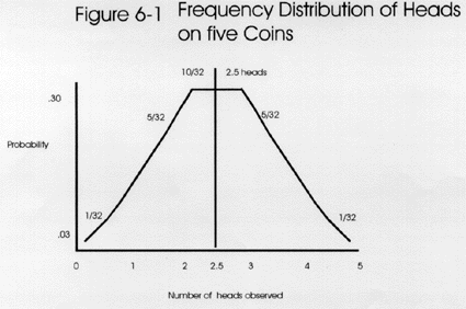
 With a 5 coin toss, it's likely to see some combinations of heads and tails based on these possible outcomes: 5H+0T, 4H+1T, 3H+2T, 2H+3T, 1H+4T, and 0H+5T. All heads would occur 1/32 times or 0.03 probability, as shown at the right. Similarly, all tails would occur 0.03 of the time. Intuitively, the greatest possibility lies in having some mixture of H and T, possibly 2.5 heads - but that number is not a reality or a real number here. The expected frequency distribution can be seen in the top figure, which shows the distribution of possibilities as fractions of 32nds. The possibilities total to thirty-two 32nds or unity. The area under the curve is greatest between 2 and 4 heads, i.e., that is the highest probability or most likely outcome.
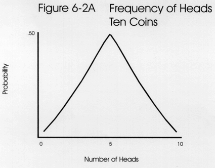
The frequency distribution for a 10 coin toss is shown in the second figure. Again, intuitively speaking, the greatest possibility is some mixture of H and T. With a 10 coin toss, achieving half heads or 5 is a real number, and the maximum probability is 0.50, as shown by the peak of the curve.
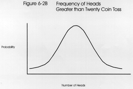
The distribution of a 20 coin toss is seen in the third figure. Again, the greatest area under the curve indicates some combination of heads and tails. When increasing the number of coins or events, the curves begin to look like normal distribution curves. As the number of events exceeds 30, the graph is considered to approximate a normal curve.
Statistical significance. The importance of this point is that a normal curve can often be used to assess the probability that an event or observed difference occurs by chance or by cause. In interpreting experimental results, it is common to use a probability of 0.05 as the cutoff between a chance occurrence and a cause occurrence. If the probability is greater than 0.05, i.e., Pr>0.05, the conclusion is that no difference exists. If Pr<0.05, then it is often concluded that a statistically significant difference has been observed; in short, that means there is a real difference due to some cause. That's why an understanding of probability is very useful for making inferences or decisions on the basis of experimental data. In the next section, we will see where that 0.05 comes from.
Standard Normal Distribution
 The standard normal distribution or the unit normal distribution is a special normal curve made up of z-scores. Remember that a z-score is a standard score (also called the standard Gaussian variable) that is calculated by subtracting the mean from a value and dividing the result by the standard deviation: z = (value - mean)/standard deviation. For example, if the mean were 100 and the value were 110, then the difference between the mean and the value is 10. If the standard deviation were 5, then the difference of 10 has 2 SD's in it, thereby it is equal to 2z.
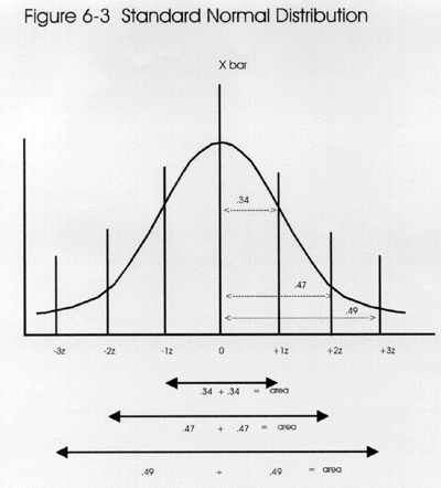
As discussed in lessons 1 and 2, this is one of those statistical forms that appears repeatedly in laboratory statistics. The formula is used to express the number of standard deviations in the difference between a value and the mean. The values for z range from zero to infinity. The figure shows that the most common z-scores are from 0.00 to 3.00. A z of 0.00 represents the mean and the range of z from +3.00 to - 3.00 encompasses almost all of the area of the distribution. In statistical language, this distribution can be described as N(0,1), which indicates distribution is normal (N) and has a mean of 0 and a standard deviation of 1.
Area under a normal curve. The total area under the curve is equal to 1.00 or unity. Half of the area, or 0.50, is on either side of the mean. The area between the mean and -1.00 z is 0.34 and the area between the mean and +1.00 z is 0.34, therefore the mean +/- 1.00z represents 68% of the area under a normal curve. The area between -2.00 z and +2.00 z is 0.47 + 0.47 or approximately 95% of the area under the curve. Between -3.00 z and + 3.00 z is 0.49 + 0.49 or approximately 99% of the area under the curve. (These numbers should seem familiar to laboratorians.) Note also that the use of +/- 2.00 z encompasses 95% of the area or a .95 probability. The remaining 1% or 0.01 probability is left in the tails of the curve. Z-scores can also be listed as decimal fractions of the 1's, 2's, and 3's we have been using thus far. For example, you could have 1.40 z's. Here the decimal fraction is carried out to the hundreths place.
Table of areas under a normal curve. It is often convenient to use a table of areas under a standard normal curve to convert an observed z-score into the area or probability represented by that score. See the table of areas under a standard normal curve which shows the z-score in the left column and the corresponding area in the next column. In actuality, the area represented in the table is only one half of the normal curve, but since the normal curve is symmetrical, the other half can also be estimated from the same table and the 0.50 on the upper half plus the 0.50 in the lower half equals 1.00 or all of the distribution.
As an example use of the table, a z-score of 1.40 is listed as having an area of 0.4192. This indicates that 41.92% of the area is between the mean or center of the distribution and the z-score of 1.40. The area beyond that particular z-score to the tail end of the distribution would be the difference between 0.5000 and the value of 0.4192, or 0.0808 because the table represents one half or 0.5000 of the area of the distribution. Now let's look at the lower half of the distribution down to a z-score of -1.40 (i.e. a negative 1.40). This too represents an area of .4192. At +/- 1.40, you would have .4192 plus .4192 or .9394 of the are under the curve. Sometimes statisticians want to accumulate all of the negative z-score area (the left half of the curve) and add to that some of the postive z-score area. All of the negative area equals .5000 plus some of the positive area, here .4192, added together would give .9142.
Here is an example of how to use the table: to find the area for a z-score of 1.96, find the value of 1.9 in the leftmost column, then find the hundredth figure from the column heading for .06, and read the area below that column, e.g., 0.4750. The area from -1.96 to +1.96 would encompass 2*0.475 or 95% of the area under a normal curve, leaving 5% outside those limits or 5% in the tails. Note that we commonly think of a 95% range as the mean plus or minus 2z or 2 SD, but that's an approximation and the exact z-score should be 1.96.
At 3.00 z, the area under the curve is 0.4987, which leaves an area of approximately 0.0013 outside in the tail. The area from -3.00 to +3.00 encompasses 2*0.4987 or 99.74% of the area, leaving only 0.26% outside. This is why 3 SD control limits have a very low chance of false rejections compared to 2 SD limits.
z-score transformation formula. The concept of the standard normal distribution will become increasingly important because there are many useful applications. If the population mean, µ, and the population standard deviation, , of any normally distributed data are known, the z-scores can be computed through the use of the following z score transformation formula:
z = (X - µ)/s
Again the formula represents the value minus the mean all divided by the standard deviation. The formula defines the difference score (X - µ or X-Xbar or delta, as seen in earlier lessons), according to how many standard deviation units it represents.
Proficiency testing example. One useful application is in proficiency testing (PT), where a laboratory analyzes a series of samples to demonstrate that it can provide correct answers. The results from PT surveys often include z-scores. For example, a glucose test value on a proficiency testing sample is observed to be 275 mg/dl. Other laboratories that analyzed this same sample show a mean value of 260 and a standard deviation of 6.0 mg/dL. In comparison to these values, our laboratory's analysis has a z-score of +2.50, which means that less than 1% of other laboratories got a higher test result (observe that a z-score of +2.50 corresponds to an area of 0.4938, which leaves only 0.0062 or 0.62% of the area in the tail above 2.50). Said another way, there is only a very small chance that the 275 mg/dL glucose value belongs with the rest of the proficiency testing values. Said another way, there is only a 0.0228 probability, or a very small chance, that the 275 glucose really does belong with the other values. Most likely it represents a measurement error by the laboratory.
z-scores vs SDs. Because there is so much confusion concerning this topic, it's worthwhile to review the relation between z-score and standard deviations (SD). The lines between statistical definitions sometimes blur over time.
Remember that the mean and standard deviation are the first statistics that are calculated to describe the variation of measurements or distribution of results. The standard deviation is a term that has the same units as the measurement, therefore it can be used to describe the actual range of measurement results that might be expected.
A z-score can be calculated once the mean and standard deviation are available. The calculated z-score [z-score = (value - mean)/SD] describes where a value is located in the distribution, e.g., a z-score of 0 is at the mean of the distribution and a z-score of 2.0 or beyond is in the tails of the distribution. Notice that SD is in the denominator of the z-score formula, so SD's and z's are not really the same. The z-score is a ratio and therefore is unitless, whereas the SD is expressed in concentration units.
But, we tend to think in terms of ±2SD as if they were ±2z. We use the SD like a z-score by saying that, if a value falls out of the curve >±2SD, then it is different from 95% of the rest of the curve (we probably should have been saying ±2z). When a value lies at >±2z's (SD's), then that value is outside of the 95% area under the curve. So 1.00 - 0.95 = 0.05. That value lies in the 0.05 area of the tails. We often use this probability of 0.05 as an indicator of statistical significance, i.e. when a value falls out >±2SD (or z's), then a statistically significant or real difference has been observed (with Pr < 0.05 that the value is a chance occurrence).
Relationship to t-distribution. In the above PT example, the population mean (µ) and the population standard deviation (s) were known quantities, i.e., the data from all laboratories participating in the proficiency testing survey were included in the calculations, thus the true mean and true standard deviation are known for the whole population. When the population mean and standard deviation are not known, which is a more typical situation, z-scores cannot be calculated. In fact, in most laboratory applications, µ and s are not known. There is, however, another family of distributions - the t-distributions - which can be used when the µ and s are approximated by Xbar and SD.
The t-distributions generally are said to have "heavier tails" as compared to the normal distribution. As the sample size gets larger and larger (N increases to about 30 or 40), these distributions begin to approximate the normal curve and can be used much like the unit normal curve because ±2t accumulates about 95% of the area under the curve. A t-value can be calculated much like a z-value, e.g., tcalc = (observed value - mean)/sXbar, where sXbar represents the standard error of the mean, which we learned about in lesson 5. If tcalc is greater than +/- 2, then a conclusion can be drawn about that particular value. A t-distribution can be used to help in making the decision that the means of two samples are far enough apart to be considered to be different, i.e., the difference is statistically significant, or close enough together to be considered the same, i.e., the difference is not statistically significant. When N is less than 30, it will be necessary to look up a critical t-value from a table.
Self-assessment questions
- What is the probability of tossing three fair coins and getting all heads? What's the probability of getting three tails? What's the probability of getting some other combination of heads and tails?
- What is a z-score?
- For a z-score of 1.65, what is the area of the standard normal curve below that value? What is the area above that value?
- How is the standard normal curve useful for data interpretation?
- If an observed difference is greater than +/- 2 z, that difference is considered statistically significant at what probability?
- Under what conditions do you use a t-distribution rather than a z-distribution?
About the author: Madelon F. Zady
Madelon F. Zady is an Assistant Professor at the University of Louisville, School of Allied Health Sciences Clinical Laboratory Science program and has over 30 years experience in teaching. She holds BS, MAT and EdD degrees from the University of Louisville, has taken other advanced course work from the School of Medicine and School of Education, and also advanced courses in statistics. She is a registered MT(ASCP) and a credentialed CLS(NCA) and has worked part-time as a bench technologist for 14 years. She is a member of the: American Society for Clinical Laboratory Science, Kentucky State Society for Clinical Laboratory Science, American Educational Research Association, and the National Science Teachers Association. Her teaching areas are clinical chemistry and statistics. Her research areas are metacognition and learning theory.
