Quality Management

A description of the variables, equations and all the mathematical details behind the Quality Planning models.

• Back to the main text of the lesson
• Conventional total error budget for stable performance
• Imprecision
• Inaccuracy
• Total Error
• Analytical quality planning model for unstable performance
• Critical-sized Errors
• Clinical quality planning model for unstable performance
• Decision Interval
• Within-subject biological variation
• Expanded models used by EZ Rules 3 and QC Validator 2.0 program
• EZ Rules 3 and QC Validator 2.0 clinical model
• EZ Rules 3 and QC Validator 2.0 analytical model
• References

Conventional total error budget for stable performance

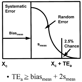
The laboratory error budget that is most commonly used today is the total error model that combines systematic and random errors as shown in the accompanying figure to produce the total error of the measurement procedure. This budget has only two components - the precision and accuracy of the measurement procedure - and it describes only the errors that are expected when the measurement procedure is working properly, i.e., stable measurement performance.

Imprecision (s_meas)

refers to the agreement between replicate measurements and is usually estimated by calculating a standard deviation or coefficient of variation from a minimum of 20 measurements on a stable material. The term "imprecision" is preferred over "precision" since the standard deviation or coefficient of variation actually describes the distribution of errors or the disagreement between replicate measurements. The term random error may also be used to describe this type of error because values are randomly higher or lower than the expected or average value. The terms stable imprecision, stable random error, and inherent imprecision are all used to indicate the performance expected when the measurement procedure is workly properly.

Imprecision is first estimated in method evaluation studies from repeated measurements on stable materials and is later estimated from ongoing measurements on the control materials being analyzed for routine QC. In evaluating performance, multiples of 2s_meas or 3s_meas are typically used as criteria for judging the acceptability of random error, however, a multiple of 4s_meas has also been recommended to provide a tighter budget for random error and allow a larger margin of safety appropriate for the QC procedures commonly used in clinical laboratories today [2].

Inaccuracy (bias_meas)

generally refers to the agreement between a measurement and the correct or true value. Inaccuracy is often used to describe the difference or bias between the values observed and the correct or true values. The term "systematic error" is also used because this type of error causes test values to be systematically high or low. The term "stable inaccuracy" is used to further clarify that this is the performance expected when the measurement procedure is workly properly.

Inaccuracy is first estimated in method evaluation studies from a comparison of results between a new method and a comparative method. The average difference between the two methods can be calculated as an estimate of bias, or the systematic difference is calculated at certain medical decision concentrations using regression statistics. This estimate can be compared to the defined allowable total error to judge its acceptability for routine application. Later on in the routine operation of a measurement procedure, inaccuracy may be estimated by the bias versus a group mean in a proficiency testing survey. We sometimes indicate this estimate by the term s_matx to distinguish it from the earlier estimate vs a comparative method.

Total error (TE_a)

describes the net or combined effects of random and systematic errors. It represents a worst case situation where a single test measurement is in error by the sum of the random and systematic components of error. Total error is usually estimated by combining the individual estimates of random and systematic errors, as shown in the following equation,

TE_a = bias_meas+ 2s_meas
where the multiplier of 2 is a z-value that determines the percent of observations that are included in the random error distribution. This multipler may be 1.65, 2.0, 3.0, or 4.0, depending on the application. Assuming bias is zero, both tails of the distribution need to be considered and a z-value of 1.65 would include 90% of the measurement distribution in the definition of TE, a z-value of 2 would include 95%, a z-value of 3 includes 99.9%, and a z-value of 4 includes essentially 100.0%. If bias were large enough so only one tail of the distribution need be considered, z-values of 1.65, 2.0, 3.0, and 4.0, contain approximately to 95%, 97.%, 99.9%, and 100% of the distribution.

This total error model for stable performance has been sometimes been used to set performance specifications for testing processes. For example, the National Cholesterol Education Program (NCEP) specifies [3] that an acceptable cholesterol method should have a 3% bias and 3% CV seem to be derived from this model. Based on an allowable total error of 9%, 3% is budgeted for bias and 6% (2s_meas) for precision. The problem is that this assumes stable performance. A method with 3% specifications will satisfy a 9% total error requirement only if it is perfectly stable and has no problems. If unstable performance occurs, analytical problems will not be detected by the QC procedures commonly used in laboratories today (3).

Note that the total error model for stable performance cannot be used to plan or select an appropriate quality control procedure because there is no QC component included in the budget. In effect, this model assumes quality control is not needed! This assumption does not seem reasonable based the widespread application of QC procedures and the accumulated evidence that testing processes are not perfectly stable. In the case of the NCEP guidelines, this assumption is contradicted by NCEP's own recommendation to perform statistical QC to monitor process performance.

More realistic error models are needed to better manage the analytical quality of laboratory testing processes. In the vernacular of the nineties, a paradymn shift is needed. A new and improved perspective can be provided by expanding the total error model to include quality control.

Analytical quality-planning budget for unstable performance

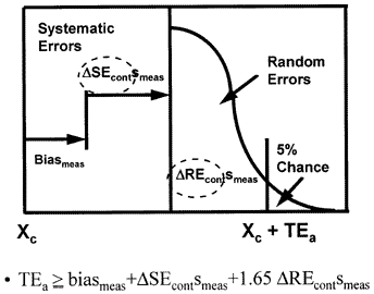
An error budget that includes the performance of the QC procedure has been described in the literature [4] and is shown in the accompanying figure.

The components of the analytical quality-planning model include the imprecision (s_meas) and inaccuracy (bias_meas) of the measurement procedure (as before) and the error detection capability of the control procedure for systematic error (?SE_cont) and random error (?RE_cont). Quality control may contribute to the overall or total variability that occurs in a test result when a measurement procedure is unstable because the control procedure has a certain sensitivity or error detection capability, i.e., errors need to be of a certain size before they will be detected. This size will vary, depending on the control rules and number of control measurements being used.

Mathematically, this analytical quality-planning model can be described by the equation shown in the figure, where ?SE_cont represents the change in systematic error that is detectable by a control procedure
?RE_cont represents the change in random error detectable by a control procedure, and the z-value is set at 1.65 to allow a maximum defect rate of 5% before the process would be declared out-of-control. The control terms depend on the particular control rules and number of control measurements used in the control procedure. The actual sizes of errors that may escape detection can be determined from power curves, which describe the probability of rejection analytical runs as a function of the sizes of errors occuring, as discussed in detail in an earlier lesson on power function graphs and critical-error graphs.

Critical-size errors

that need to be detected by QC can be calculated from the analytical quality-planning model, as follows. For the critical systematic error that needs to be detected, set ?RE_cont= 1.0, then solve for ?SE_cont, which gives the following equation:

?SE_crit = [(TE_a - bias_meas)/s_meas] - 1.65

For the critical random error that needs to be detected, set ?SE_cont to 1.0, then solve for ?RE_cont, which gives the following equation:

?RE_crit = [TE_a - bias_meas)/1.65s_meas

When a z-value of 1.65 is used, these equations are the same as those used earlier in the QC planning process [see QC planning applications].

This analytical quality-planning model allows the laboratory to budget for safe operation. By including QC performance, the analytical process can be designed or planned to have the correct balance of imprecision, inaccuracy, and QC. Most often this is done by estimating the imprecision and inaccuracy that are present, then selecting the QC rules and N needed to detect the critical systematic errors. However, you can also specify the QC you want to use and then determine the specifications for imprecision and inaccuracy that are needed to maintain adequate control in routine operation. In this way, you can set specifications for purchasing new methods that will provide cost-effective operation in your laboratory.

The main limitation of the analytical quality planning model is that it does not directly relate the measurement and control specifications to the clinical needs of the test. We can assume that the total error criteria utilized in proficiency testing programs represent clinical needs and should provide adequate guidance for planning our testing processes, but it is also desirable to be able to develop these specifications directly from clinical requirements.

Clinical quality planning budget for unstable performance

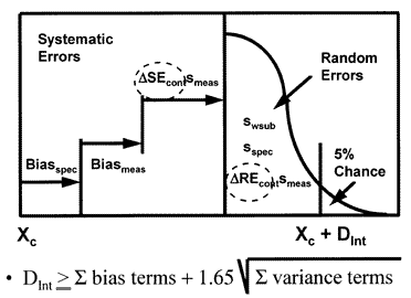
A clinical quality planning model that incorporates both preanalytical and analytical components [5] is shown here.

This model is more complicated, as expected, because it includes more factors that affect the variation of a test result. For example, additional bias may occur due to the specimen type or condition; additional variability may be caused by sampling, as well as the subject's own biological variation.

To mathematically combine all these error components, systematic error terms are added algebraically whereas random error terms are squared, added, then the square-root extracted. This gives the general form of the equation shown in the figure, and the specific form shown below:

D_Int = bias_spec + bias_meas + ?SE_conts_meas + 1.65[s²_wsub + s²_spec + (?RE_conts_meas)²]^1/2

where D_Int is the clinical decision interval,
bias_spec is the sampling bias,
bias_meas is the analytical measurement bias (stable inaccuracy),
s_meas is the analytical measurement imprecision (stable imprecision),
?SE_cont is the sensitivity or change in systematic error (unstable inaccuracy) to be detected by the QC procedure,
z-value of 1.65 is related to the maximum allowable defect rate or chance of exceeding the quality requirement before a run is rejected, which is set at 5% here,
s_wsub is the within-subject biological variation,
s_spec is the between-specimen sample variation,
and ?RE_cont is the change in random error (unstable imprecision) to be detected by the QC procedure.

Decision interval (D_Int)

corresponds to the gray zone between two different test values that would lead to different actions in response to a test result. For example, the NCEP guidelines for interpretating a cholesterol test recommend that a value of 200 mg/dL or less requires no action and that a value of 240 mg/dL or more requires follow-up testing to diagnose the cause of the elevation. This gray zone from 200 to 240, or 20% at a decision level of 200 mg/dL, defines the quality required for the clinical use of the test. In managing a cholesterol testing process, a laboratory should be sure that a specimen from a patient whose true homeostatic set point is 200 mg/dL will not be erroneously reported as a value of 240 mg/dL. Both analytic and pre-analytic errors need to be considered to properly manage the testing process.

Within-subject biological variation (s_wsub)

describes the patient's own variation about a homeostatic set point. For cholesterol, for example, s_wsub is approximately 6.5%. A patient whose true homestatic set point is 200 mg/dL (5.17 mmol/L) would have a 95% range of 174 to 226 mg/dL (or 4.50 to 5.84 mmol/L). Over half of the NCEP decision interval is consumed by within-subject biologic variation. All the other preanalytical and analytical components must fit within the remainder of the budget.

Within-subject biologic variation may add to any analytical variation to further complicate the interpretation of a test result. For cholesterol, the within-subject biological variation of 6.5% is considerably larger than the NCEP 3% specification for s_meas, therefore, biological variation will actually be the dominate component that limits the physicians' interpretation of cholesterol test results. The combined variation due to the biological and analytical components is expected to be about 7.2%, which is only a small increase over the 6.5% biological variation itself.

Through experience, physicians acquire a feeling for the magnitude of the combined biological and analytical variation and often develop some guidelines for the changes that are medically important. These judgments of medically important changes provide a source of information about customer expectations or quality requirements for laboratory tests. Clinical vingettes have sometimes been used to obtain a collective judgment of medically significant changes, which have then been used to estimate medically allowable SDs or CVs. In making such estimates, the biologic component needs to be deducted, otherwise, the allowable analytical variation will be too large. Some of the widely referenced estimates of medically allowable CVs have not deducted biological variation, thus this mistaken theory has led to the myth that laboratory performance today is better than needed for clinical purposes.

Expanded models used by QC Validator 2.0 and EZ Rules 3 programs

These quality planning models can be expanded to consider additional factors, such as the number of tests, number of specimens, and number of replicate samples analyzed. These expanded models are the ones used by version 2.0 of the QC Validator program. The models in version 1.1 of the program are very similar, but do not fully consider the effects of the number of replicate samples. However, in most applications, the number of tests, specimens, and replicate samples are set equal to 1, in which case the models behave the same. For non-computerized applications or even spreadsheet applications, the simpler forms of the models (as described earlier) may be more practical.

QC Validator 2.0 clinical model

The clinical model is shown below:

In this model, bias_matx is the measurement bias due to matrix effects, n_test is the number of tests performed, n_spec is the number of specimens drawn for each test, and n_samp is the number of samples measured for each specimen. The impact of biological variation could be reduced by performing multiple tests, specimen variation could be reduced by drawing multiples specimens, and analytical variation could be reduced by analyzing replicate samples. For improving the clinical usefulness of cholesterol testing, for example, it may be more valuable to perform two different tests to reduce the biological variation, rather than making replicate measurements to reduce method imprecision (3).

Note that bias_meas and bias_matx are combined and presented as bias_totl on the y-axis of the OPSpecs charts prepared by the program. Bias_totl is the sum of bias_meas plus bias_matx, which are the individual bias terms that can be entered in the parameters screen of the EZ Rules 3 program. Also note that the computer program allows entry of two different terms for analytical bias - bias_meas as defined earlier and bias_matx which represents bias due to or estimated from matrix materials. When we originally described the quality-planning models, we thought it would be useful to have different inputs for the estimates of bias obtained from method validation studies and proficiency testing surveys, thus we included two bias terms. This has been very confusing for a lot of analysts, so in the future, we will probably drop the bias_matx entry and just use bias_meas for any estimate of bias, regardless of the experimental design or source of data. In practice, we usually enter a bias-value as bias_matx when using an estimate from a proficiency testing survey and then leave bias_meas as zero. We enter a bias-value as bias_meas when the estimate comes from a method evaluation study, such as the comparison of methods experiment.

QC Validator 2.0 analytical model

An important feature of the quality-planning models described here is the logical consistency between the clinical and analytical models. For example, if you set all the preanalytic terms to zero in the clinical quality planning model, you end up with the analytical quality planning model. If you assume stable performance and set ?SE_cont to 0.0 and ?RE_cont to 1.0, you end up with the analytical total error model for stable performance. This should give you some confidence that the error budgets being constructed are correct and also some understanding that they can be updated and improved.

For example, the expanded clinical model that considers the number of tests, specimens, and samples can be reduced to an analytical model by setting the preanalytical terms to zero, giving the following equation:

TE_a = bias_meas + bias_matx + ?SE_conts_meas/(n_test)^1/2 + z?RE_conts_meas/(n_test)^1/2

When the interest is detection of systematic error, RE can be set to 1.0, i.e., and the equation reduces further:

TE_a = bias_meas + bias_matx + [?SE_cont+ zs_meas]/(n_test)^1/2

This provides an analytical model that can be used to assess the effects of making replicate measurements, as well as the effects of improvements in the imprecision and inaccuracy of the measurement procedure. Of course, making replicate measurements is one way of reducing imprecision, but this approach could be costly in the long run compared to actually reducing the SDs or CVs through methodological improvements.

Note again that bias_meas and bias_matx are combined as bias_totl when OPSpecs charts are prepared by the program, as pointed out in the discussion of the clinical model.