Z-Stats / Basic Statistics

Enough of this abstract statistical stuff: how do we use these things in the laboratory? This article shows you the practical application of statistics on the bench-level, including how to find the bias and other important stats.

EdD, Assistant Professor
Clinical Laboratory Science Program, University of Louisville
Louisville, Kentucky
October 2000

• Review of the regression model
• Standard error of regression and random error
• Y-intercept and constant systematic error
• Slope and proportional systematic error
• Bias and overall systematic error
• Problems with regression
• References

In the previous lesson, we described regression in the classical fashion. In this lesson, we will describe practical laboratory applications and some of the complications encountered when working with real experimental data. The language and applications of regression are all around us in the laboratory, particularly in the established practices for method validation and quality control. Terms such as Bias, (Ybar-Xbar), [(bXbar + a) - Xbar], slope, intercept, and S_y/x to name just a few, all derive from regression terminology. In this lesson, we will illustrate how regression statistics can be used to estimate the analytical errors occurring with a laboratory method. We'll focus on a comparison of methods experiment, which is commonly used to validate that a new method provides results consistent with the old method that is being replaced.

Review of the regression model

In the last lesson, we looked at the derivation of the slope coefficient of the regression line from the deviation scores of the X and Y variables. The regression line provides an equation that can be used to predict Y from X (Y=bX + a). Most often the data points that depict the "real Y" or Y-observed do not lie on this regression line, therefore it is important to quantify the explained and unexplained components. To do this, we considered several Ys, including the grand mean of Y, the Y-predicted-from-X, and the Y-observed in the data point. In the diagram of The Several Ys, the distance from Y' or the Y-predicted-from-X to the grand mean was called Y-explained or Y-regression. The distance from Y' to the Y- observed was called Y-error, which is often shown in a scattergram by the vertical distance or lines drawn from the data points to the regression line.

In our mathematical calculations, we then developed five more columns (C-8 through C-12) that represented the calculations of Y-predicted, Y-residual or error, Y residual squared or error sum of squares (ESS), Y-explained or Y-regression, Y-explained squared or regression sum of squares (RSS). Adding ESS and RSS yielded a total sum of squares or TSS. R square or the variance in Y-explained by the regression was the ratio of the regression SS divided by the TSS. The larger this number, the more efficient X is in predicting Y. For example, if R² = 0.80 then we are doing 80% better at predicting Y by using X then we would do predicting Y by using the mean of its own distribution. In this way, regression can be used to describe the strength of a relationship between X and Y.

Interestingly 1-R² is the variance in Y not explained by X. This term is also called tolerance, Wilk's lambda and has other names. It is equal to the Error SS divided by the TSS.

Standard error of regression and random analytical error (RE)

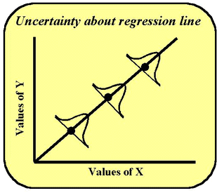
As usual, we need to look at some standard error terms. In observing a "best fitting line" in the least squares approach, for each Y-predicted from a particular X, there is a best estimate involved. The line is approximated such that each Y observed value is estimated at its least squared distance from the line. However, even with this predicted Y, there is always some uncertainty (probability) about just where each Y is in relation to its X. Because of this a mini-normal distribution can be drawn around each point on the regression line, as illustrated in the accompanying figure.

The dot on the line appears at the most likely point in that frequency distribution--at the mean. This mini-distribution represents the standard error about the regression line called the SD of the regression line or the standard error of the estimate or s_y/x. This statistic should be included as part of the regression calculations for any comparison of methods experiment to provide an estimate of the random error between methods. Note that this estimate will include the random error of both methods, plus any systematic error that varies from sample to sample (e.g., an interference that varies from sample to sample). Therefore, it is expected to be larger than the imprecision of the test method and is not a substitute for the imprecision determined for data from a replication experiment.

This variation about the regression line also gives us information about the reliability of the slope and intercept because additional terms can be calculated for the standard error of the slope, called S_b, and the standard error of the intercept, called S_a. Computer programs may use these terms to calculate confidence intervals for slope and intercept. Ideally, a regression between two test methods should have a slope of 1.00 and an intercept of 0.0. The significance of small deviations from the ideal slope and ideal intercept can be assessed using S_b and S_a to calculate the confidence intervals about the observed slope and intercept. If the intervals overlap the ideal values, the differences from ideal are not of any practical importance, i.e., they're not statistically significant. (Ideal means that 1.00 is found in the slope interval and 0 is found in the intercept interval.)

Y-intercept and constant systematic error (CE)

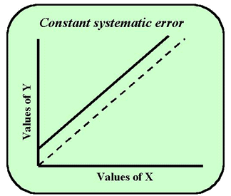
In comparing two methods, x and y using regression, let's look at what would happen if the intercept of the regression line were not at the 0,0 point for x and y, as shown in the next figure. The dashed line represents ideal performance. The solid line does not pass through 0,0 or the origin of the graph. Rather it does not ever register a zero value on the y-axis. The reason for this is that the regression equation here is not y = 1x + 0. Rather the formula is something like y = 1x + 3. That is, the constant in the formula (a) is something other than zero. When x is zero, y will be the number three. Therefore the line does not cut the y-axis at the zero point but at the 3 point. The constant term in the regression equation shows a deviation or error from the ideal value of zero. Such a problem is usually due to some type of interference in the assay, inadequate blanking, or a mis-set zero calibration point. It would be useful to test the confidence interval around the constant using s_a. If zero falls within the confidence interval, then the deviation is not important. If zero does not fall with the interval, then the deviation reveals a constant systematic error between the methods.

Slope and proportional systematic error (PE)

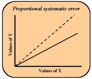
In testing two methods, x and y, let's look at what would happen if the slope of the regression line were not one. In the figure here, the dashed line represents a perfect 1:1 relationship between x and y. The intercept is at 0.0 and the slope of the line makes the 45 degree angle with the base of the graph. For every increase of one in x, y also increases by one. The solid line shows a lower slope, e.g., this line represents a regression equation such as y = 0.8x + 0. Here for every x increase of one, y increases by a factor of 0.8. It would be useful to test the confidence interval around the slope using S_b. If a value of 1.0 falls within the confidence interval, then the deviation is not important. If 1.0 does not fall with the interval, then the deviation reveals a proportional systematic error between the methods. Something is wrong that causes a loss of proportionality with y. This type of error whose magnitude increases as the concentration of analyte increases is often caused by poor standardization or calibration. Sometimes it is caused by a substance in the sample matrix that reacts with the sought-for analyte and therefore competes with the analytical reagent.

Bias and overall systematic error (SE)

The overall systematic error is often considered to be a bias between test procedures, which implies that one method runs higher or lower than the other. As discussed in earlier lessons, bias can be calculated as part of t-test statistics and provides an estimate of the average difference between the values obtained by the two methods, or the difference between the averages of the two methods for a series of specimens. It is important to understand that this estimate of bias would apply at the mean of the data, i.e., it represents the average or overall systematic error at the mean of the data.

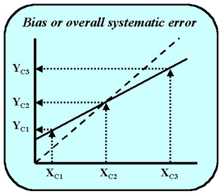
If it were of interest to know the overall systematic error at a medically important decision concentration, X_C, that is not at the mean of the data, then the regression equation becomes useful. For example, the test results for a glucose method would be critically interpreted at several different decision levels, such as 50 mg/dL for hypoglycemia, 110 mg/dL for a fasting glucose, and 150 mg/dL for a glucose tolerance test. To estimate the systematic errors at these three medical decision concentrations, it is advantageous to use regression statistics. The value for Y that corresponds to the medical decision concentration, Y_C, is calculated from the regression equation, Y_C = bX_C + a. The difference Y_C - X_C represents the systematic error at the medical decision level of X_C.

For example, in the figure shown here, there are three medical decision concentrations that are important in the interpretation of a test. The systematic error at a high medical decision level, X_C3, is negative, i.e., the y-values are lower than the x-values at high concentrations. At the low medical decision concentration, X_C1, the y-values are higher than the x-values, giving a positive systematic error. In the middle of the range, there is no systematic error. If the method comparison data were analyzed by t-test statistics and the mean x-value fell in the middle of the range, no bias would be observed, even though there obviously are systematic differences at low and high concentrations.

Problems with regression

As noted in earlier lessons, there are certain assumptions that should be satisfied in regression analyses:

• A linear relationship is assumed;
• X-values are assumed to be "true" and free of error;
• Y-values are assumed to show a gaussian distribution;
• Random error is assumed to be uniform over the range of the data studied, i.e., there is an assumption of homoscedasticity, which means the variance of y is assumed to be the same for each value of x.
• Outliers - individual points that do not seem to fit the general distribution or scatter in the data - can seriously affect the values of the slope and intercept.

Regression applications with real laboratory data may have any or all of these problems! Here are some practical ways to deal with them.

Linear relationship. Examine a plot of the data to assess whether there is a linear relationship. Pay particular attention to the high and low ends of the data. If necessary, restrict the statistical analysis to the data that shows a linear relationship

Error in x-values. There will always be some error in the x-values if they are measurements from a comparative method, even if that method is very precise. The errors will not bias the regression statistics as long as the range of data is wide relative to the imprecision of the comparative method. The correlation coefficient provides a convenient indicator. If r is 0.99 or greater, there is no worry about the effect of error in the x-values. If r is less than 0.95, then extra care needs to be taken. This might involve collecting additional data to extend the range studied and achieve a higher r-value. Or, it might involve the use of alternative statistical calculations, such as t-test anlaysis if the mean of the data is close to the medical decision concentration of interest, or a more complicated regression techniques, such as Deming's regression [1]. Note that one or a few high or low points can have a large effect on the value of the correlation coefficient, therefore it is useful to inspect a plot of the data and be sure that the data covers the range in a fairly uniform manner.

Gaussian distributions. In the case of a comparison of method experiments, the y-values are measurement values and are expected to be gaussian. Note that the requirement for gaussian values is not for the patient distribution, but for the distribution of measurements that would be obtained on individual patient samples. That assumption is reasonable because we're dealing with measurement variation, not population variation (where it would not be reasonable).

Homoscedasticity. The most important thing is to learn to say this word so you can sound like a statistician. In practice, the assumption is violated by most methods, but not so seriously as to require changing to alternative calculations, such as weighted regression. The NCCLS EP9-A protocol for method comparison studies [2] recommends making a visual check for uniform scatter to determine if there are any dramatic and significant differences between the scatter at the upper and lower ends. This protocol uses 3:1 as a guideline, meaning that it's okay as long as the scatter at the high end is less than 3 times the scatter at the low end.

Outliers. Individual points near the ends of the range can exert undo influence on the values of the slope and intercept. Think of the regression line as a teeter-totter that balances on the mean of the x and y values. A single point that is far off the line exerts more weight when it is near the end of the teeter-totter, pulling the line in that direction. A high point at the high end of the range will pull the line up, causing the slope to increase and the intercept to decrease (teeter-totter effect). As low point at the high end of the range will pull the line down, causing the slope to decrease and the intercept to increase. A simple way to spot outliers is to inspect a plot of the comparison data. Some people prefer to use a difference plot for this purpose, or a plot of the residuals about the regression line. Removing outliers requires great care because you're tampering with the data set. It's best to re-test the sample and confirm that a mistake was made before removing any data point. Problems with outliers can be minimized by making duplicate measurements, carefully inspecting and plotting the data at the time it is collected, and re-testing discrepant results while the specimens are still available.

For additional discussion on the use of regression statistics in method comparison studies, see MV - The Data Analysis Toolkit and Points of Care for Using Statistics in Method Validation on this website. Note that a regression calculator is available as part of the Paired Data Calculator in the Data Analysis Toolkit on this website.

References

1. Cornbleet PJ, Gochman N. Incorrect least-squares regression coefficients in method comparisons. Clin Chem 1979;25:432-438.
2. NCCLS. Method comparison and bias estimation using patient samples: Approved Guideline. NCCLS document EP9-A. NCCLS, 940 West Valley Road, Suite 1400, Wayne, PA 19087.