Z-Stats / Basic Statistics
Z-13: The Least Squares Regression Model
More on scattergrams, variables independent and depente, variances explained and unexplained, and deviations squared and unsquared.
EdD, Assistant Professor
Clinical Laboratory Science Program, University of Louisville
Louisville, Kentucky
August 2000
- Predicting Y from X
- Understanding the regression model
- Calculating the regression slope and intercept
- Several Ys and various variances
- Unexplained error variance and the standard error (sy/x)
- Explained variance and the coefficient of determination (R²)
- Null hypothesis in regression
- References
In the last lesson, we saw that the correlation coefficient could be used to describe a relationship between a dependent and independent variable, but that we should not rely too heavily on those results. We also looked at the formula for a straight line and saw how regression could be used to draw a straight line through the data in a scattergram. From regression, we had additional information about the slope of that line and the y-intercept, which should be useful in comparing the results from two different analytical methods.
In this lesson, we will look more closely at the way the various terms used in regression are related. We will cover regression in the classical fashion and will derive a measure of strength of relationship (one of the most important concepts in statistical analyses). Much of the coverage concerns mathematical operations that we have used over and over again.
Predicting Y from X
In Lesson 12, we considered a container full of Y values and a container full of X values. We were given the opportunity to pull out a Y value, however we were asked to guess what this Y value would be before the fact. The best guess would be the mean of all the Y values unless we had some additional information, such as the relationship between X and Y. Regression gives us the information to use the X values to estimate what the corresponding Y values should be. In other words, we can predict Y from X! And, by using X to predict Y, we will get closer to any particular Y than by just guessing Y's mean.

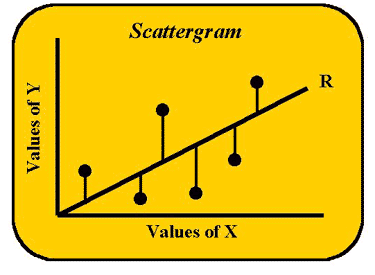
Let's start with the scattergram shown here to develop a concrete image of what regression is all about. We are going to look at the actual Y values and Y-predicted-from-X values. The individual data points appear as X and Y coordinates. The Y-coordinates of the points are the true Y values. The line represents the regression of Y on X or the Y-predicted-from-X values. If each and every one of the data points were to lie exactly on this line, we would have perfect correlation between the X and Y values. However, that is not what we see in this figure.
The lines extending up or down from each data point to the line, or the vertical distances between the points and the line, represent the error in estimating Y from X or the differences between what Y actually is and what X predicts it to be. The least squares approach to regression is based upon minimizing these difference scores or deviation scores. The term deviation score should sound familiar. These are the same deviation scores discussed in earlier lessons with the exception that, instead of just X's deviations, Y's deviations are now going to be considered as well. First we need to do some mathematical "housekeeping" to keep everything straight. The deviation scores can also be represented in script or italics.
X's deviations = X-Xbar = x
Y's deviations = Y-Ybar = y
Also the italic terms can be multiplied by each other. The cross product of x and y is xy or the cross product of the deviations of X and Y. In the least squares model, the line is drawn to keep the deviation scores and their squares at their minimum values.
Understanding the regression model
To develop an overview of what is going on, we will approach the math in the same way as before when just X was the variable. In the accompanying table, we define seven columns (C 1-7) of familiar form, e.g., columns C1, C3 and C6 represent what we have done with X in prior lessons.
| C1 | C2 | C3 | C4 | C5 | C6 | C7 |
| Independent variable |
Dependent variable |
Deviation Score for X |
Deviation Score for Y |
Cross Product |
Deviation Squared |
Deviation Squared |
| X | Y | X-Xbar or x | Y-Ybar or y | xy | x² | y² |
| 6 | 8 | 1 | 2 | 1*2=2 | 1² = 1 | 2² =4 |
| 7 | 9 | 2 | 3 | 2*3=6 | 2²=4 | 3²=9 |
| . | . | . | . | . | . | . |
| SX | SY | Sx = 0 | Sy = 0 | Sxy | Sx² or SSX | Sy² or SSY |
| Xbar=5 | Ybar=6 | 1st moment Pearson correlation | 2nd moment | |||
Column 1 (C1) shows X as the independent variable or predictor variable values. The sum of the X-values is used to calculate the mean or Xbar, which has a value of 5 as shown at the bottom of C1. C3 shows the deviation or difference of individual X-values and the mean of X, which is a difference score like those seen in prior lessons. The value is referred to as script x or italic x. (It is important to recognize that the sum of the first set of difference scores, C3, always equals zero. This is the Pearson "first moment.") Skipping to C6, this column gives the square of X's difference scores from the mean of X, and the sum of script x squared is called Pearson's second moment or sum of squares (SS) that we have seen many times before.
Now we will do the same types of manipulations for Y starting with C2, which shows the values for Y or the dependent variable, the sum of Y, and the mean. C4 represents the deviation scores for Y from its mean, again script y or y, and the sum is always zero, a first moment. C7 represents the square of Y's difference scores from the mean of Y and gives the sum of script y squared called the second moment or SS. C5 holds the cross product of the X and Y difference scores or script x times script y or xy.
Calculating the regression slope and intercept
The terms in the table are used to derive the straight line formula for regression: y = bx + a, also called the regression equation. The slope or b is calculated from the Y's associated with particular X's in the data. The slope coefficient (by/x) equals:

Or using the columns:

Again, these formulae represent the slope of the line or b of the straight line formula: Y = bx + a. To estimate the a or the y-intercept, the mean values for x and y can be entered into the equation along with the calculated slope:![]()
where Ybar and Xbar are calculated from the summations of C2 and C1, respectively.
Several Ys and various variances
We need to examine more closely what is happening with the dependent variable Y. There really are several Y's to be considered, which are not immediately obvious. Remember the scattergram shows points representing actual x,y coordinates for observations, as well as a straight line that comes from the regression formula.
- For each X value, there is a corresponding observed or measured Y value, i.e., there is a (concrete, actual) Y observed (Yobs). Usually this Y does not lie on the line.
- There is a second Y for each X. It is the Y found on the regression line itself, and it also is the Y predicted from the formula y = bx + a. Y-predicted is represented several different ways in the literature: Y prime, Y' or Y with a caret(^) called Yhat. Y' will be used here as the predicted Y.
- The third Y is the calculated Y mean, the mean of the Y distribution, or Ybar, and in this case it will also be called Y Grand Mean or YGM. Remember, if you had to predict what any one Y is, the best guess is the mean of the Y distribution.

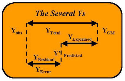
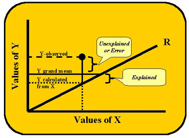
The accompanying figure shows the relationships of The Several Ys. The top line diagram is actually showing the difference between the real or observed value (Yobs) and Ybar or the grand mean of the distribution (YGM). This distance between Yobs and YGM is called the "total" distance or YTotal. Intervening between these two values is the value for Y that can be predicted from the (regression) equation using X's value, i.e., Y' = bX + a. The distance from Y' to YGM is explained by the regression equation, so it is called YRegression or YExplained (and sometimes confusingly YPredicted). The "leftover" or unexplained distance from Y' to Yobs is the residual or error of the estimate. The relative lengths of these lines provide a comparison of the explained and unexplained variation. If the length of the line from Y' to YGM is longer than from Y' to Yobs, then regression is doing a better job of predicting Y than just guessing the mean of Y.
Unexplained error variance and the standard error (sy/x)
To provide more quantitative terms for the unexplained and explained variation, we need to calculate some more sums of squares, as shown in the following table.
| C8 | C9 | C10 | C11 | C12 |
| Y Predicted Y' |
Residual or error (Yobs - Y') |
Residual squared (Yobs - Y')² |
Y Explained (Y' - YGM) |
Explained squared (Y' - YGM)² |
| 2 | 4 | 4² = 16 | 1 | 1² = 1 |
| 3 | 3 | 3² = 9 | 2 | 2² = 4 |
| . | . | . | . | . |
| . | . | . | . | . |
| Sresidual or error sum of squares ESS |
Sregression sum of squares RSS |
Column C8 shows the Y values predicted for each particular X using the regression equation. C9 represents the difference between the observed Y and the predicted Y. Since this amount could not be predicted using the regression equation, i.e., it is unexplained, the quantity is called the residual or error term. C10 shows the square of this error term and the sum of the column gives the error sum of squares (ESS). This variance can be used to calculate the standard error of the regression line (sy/x), sometimes also called the standard deviation of the residuals or standard deviation of the points around the regression line:
sy/x = (ESS/N-2)1/2 = (![]() C10/N-2)1/2
C10/N-2)1/2
where N-2 accounts for the loss of 2 degrees of freedom due to the previous calculation of the slope (b) and y-intercept (a).

Explained variance and the coefficient of determination (R2)
Continuing in developing sums of squares, C11 is the predicted Y (Y') minus the mean of Y's distribution (YGM), which is called Yexplained. C12 holds the square of the values in C11. The sum of values in C12 is called the regression sum of squares, regression SS (RSS), or the sum of squares explained by the regression equation. Finally, there is one more sum of squares that needs to be examined, the total sum of squares (TSS) that represents the longest line in the figure showing the several Ys. It is equal to the regression or explained sum of squares plus the residual or error sum of squares that is unexplained.
TSS = Regression SS + Residual or Error SS
(Yobs-YGM)² = (Y'-YGM)² + (Yobs-Y')²
TSS = RSS + ESS
Now we will define a new term, the coefficient of determination or R2, that is the ratio of the RSS (explained in the regression) divided by the total SS or:
R2 = RSS/TSS
R2 gives us a way to see how much of the sum of squares was explained by the regression. In fact, instead of talking about SS or sum of squares, we can now talk about the "variance explained." (However, remember SS divided by N gives the variance term) We are now saying that:
R2 or r2 = (explained variance)/(total variance)
And we can actually talk percentages. Let's say that R2 = 0.95, which means that the ratio of variance explained by X to the total variance is 0.95. Multiply by 100 to make it a percentage, i.e., 95% of the variance is explained. Now in relation to our earlier cholesterol example, we can say that we are doing 95% better predicting a cholesterol value using a person's age than we would do predicting cholesterol by using its own central tendency or mean. In the case of method comparison, method X explains 95% of the variance in method Y. And the remainder of the 5% of the variance in the dependent variable Y was not explained by the variance in X, therefore it is error. (This 5% comes from 100%-95% or 1.00-0.95. Remember when we looked at "little r" and "little r square" in correlation, its largest value was 1.00? The same applies here.)
This error variance also has a particular way of being expressed. Let's rearrange the formula.
RSS + ESS = TSS
RSS = TSS - ESS
Since TSS-ESS can be used to replace RSS, often the R2 formula looks like this:
R2 = RSS/TSS = (TSS - ESS)/TSS = 1 - ESS/TSS
(Remember R square's largest value is 1.00)
The remainder or unexplained variance, which is also called Wilk's lambda, can then be written as:
ESS/TSS = 1 - R2
In the above examples, we were able to explain 95% of the variance in Y by using X. In this way, regression can help us to see the strength of a statistical relationship or how much variance is explained in the dependent variable by the independent variable. The greater the R2 (up to 1.00) the more variance is explained by the regression. That is how much better we can do at predicting the dependent from the independent. This R² is a proportional reduction in error (PRE) coefficient and gives us an idea of the effect size (ES) of our independent variable. Examining ES is better than significance testing because it is less sensitive to problems of sample size (N).
Null Hypothesis in Regression
Oftentimes computer printouts for regression will list a probability. Remember whenever there is a probability, you need to stop and ask yourself what null hypothesis is being tested. The Ho in regression is: No linear relationship exits between (among) the variables. We usually want to overturn this Ho. It is expressed this way: Ho: b = 0. Now we need to explain this beta. Remember the regression formula is: y = bx + a, and b is the slope coefficient. There is a way to convert b using z-scores. When this is done, b is called b or the standardized slope coefficient. Now we will substitute b into the formula: y = bx + a. If the null hypothesis were true and b = 0, then y = (0)x + a and there is no linear relationship between y and x. In fact y=a or the constant at all times. Usually we want to find a relationship and a strong one at that. We will look at more of these relationships in the next lesson.
References
- Kleinbaum, D. G., Kupper, L. L. & Muller, K. E. (1988). Applied regression analysis and other mutivariable methods, 2nd ed. Boston, MA: Kent.
- Tabachnick, B. G. & Fidell, L. S. (1996). Using multivariate statistics, 3rd ed. New York, NY:HarperCollins.
